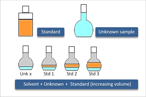
Standard addition is a quantification approach (similar to ESTD or ISTD) useful in case the sample matrix is complex and when it influences responses of analytes. By spiking samples with a series of increasing amounts of the analytes, standard addition calibration curves for each sample are obtained from which the concentrations of unknown samples can be calculated.
- Create a new method or open your already prepared method. Go to Method Setup - Calculation tab.
- Create New calibration file ⓐ or Set your already created Calibration file ⓑ.
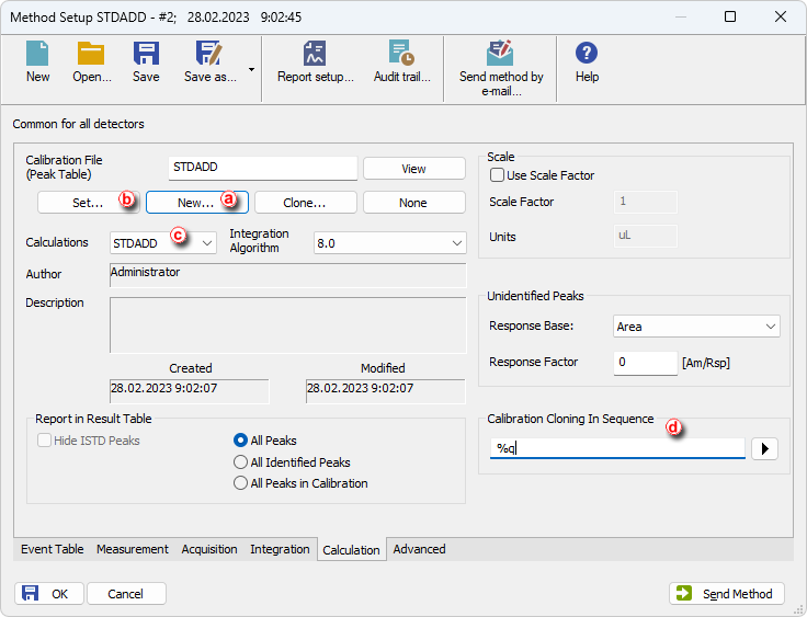
- Select STDADD in the Calculations drop-down list ⓒ.
- Create a custom name for the cloned calibration files in Calibration Cloning in Sequence ⓓ and click OK.
- Open the Calibration window by selecting Window - Calibration in the Instrument window.
- Open the Calibration Options dialog. Choose Calibration - Options… or click on
 . Select the STDADD in the Display Mode drop-down list and click OK.
Note:
Make sure that each of the measured samples will have a unique calibration name; use predefined parameters to achieve that.

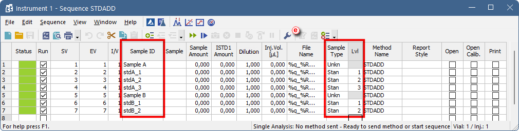
- Create a new sequence with the given order of the lines:
- Sample A
- Sample A with Standard level 1
- Sample A with Standard level 2
- Sample A with Standard level X
- Sample B
- Sample B with Standard level 1
- Sample B with Standard level X
- continue with the given pattern until desired state
- Set the columns as follows: for Unknown samples set Sample Type column to Unknown and for Standard Addition samples, set Sample Type column to Standard and Lvl column to level corresponding to the added amount in given sample.
Note:
In case you want to use a blank sample too, such sample shall be always put in the sequence before the unknown sample.
- Click
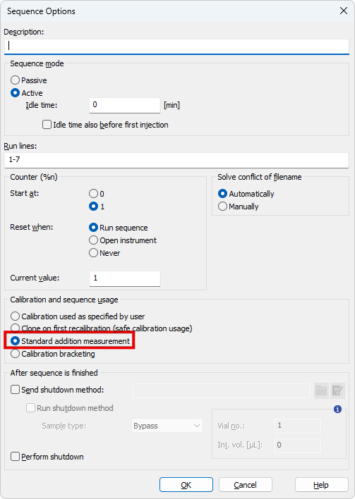
 to open the Sequence Options dialog ⓔ and select Standard Addition Measurement and click OK.
- Run the sequence and wait until the sequence is finished.
- Open the Calibration window: choose Window - Calibration in the Instrument window or click on
 .
. - Go to File - Open and open the cloned calibration file for the desired sample.
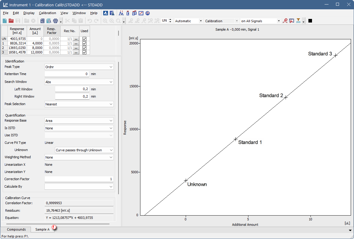
- Click on the Compound tab ⓕ to see the calibration curve. Fill in the amounts of the standard samples.
- Open chromatogram of the desired unknown sample. The Result Table now contains amount of the unknown sample, calculated using Standard Addition.
Note:
The measured sequence can be reprocessed using Batch. For more info see the topic Reprocessing whole sequence while using calibration cloning.
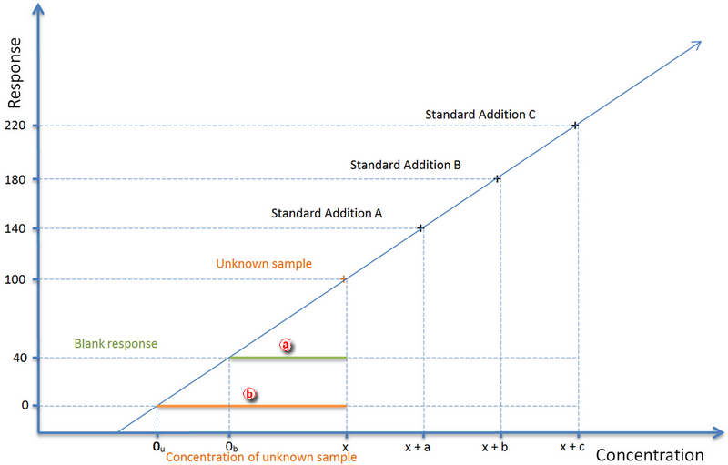
How the concentration is calculated
The concentration of an unknown sample is calculated using a calibration curve, which intersects in the point [0,0].
As shown in the picture below, when not using Blank samples the the concentration of an unknown sample equals the orange line (0 response corresponds to 0 unknown sample concentration - 0u), whereas the concentration of the UNKNOWN SAMPLE when using Blank equals the green line (Blank response corresponds to 0 unknown sample concentration - 0b).